Introduction

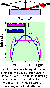
This page is a CGI interface to my program TRDS_sl simulating non-specular x-ray scattering from multilayers with interface roughness. The basic ideas of this field are formulated in the famous work by Sinha et al [1]. The angular pattern of non-specular scattering is related with the Fourier transform of roughness spectrum (Fig.1). Therefore, the measurements can bring the correlation function of statistical roughness distribution. 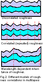In recent years this technique has found widespread applications in the studies of roughness inheritance and interface-interface correlations in multilayers [2-12] (Fig.2). 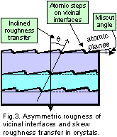These measurements are especially valuable for semiconductor multilayers where the roughness anysotropy, the skew roughness correlations between interfaces, and the distributions of atomic steps on vicinal interfaces can be investigated [13-18] (Fig.3).

TRDS_sl implements a number of different models or roughness in multilayers suggested by different authors. These include wavelength-dependent and asymmetric roughness correlations between different interfaces and roughness due to atomic steps on vicinal interfaces. The diffuse scattering is calculated in the distorted-wave Born approximation (DWBA) with the wavefields of non-rough reflector provided by TER_sl. The calculations are for coplanar scheme of measurements (Fig.1) most often used in the experiments. (the scattered radiation is integrated over the deviations from the reflection planes). The differential schemes [9,10] with out-of-plane resolution are not supported by this version of the program.

1. S.K.Sinha, E.B.Sirota, S.Garoff, and H.B.Stanley, "X-ray and neutron scattering from rough surfaces", Phys. Rev. B, 38 (1988) 2297-2311.
2. A.V.Andreev, A.G.Michette, and A.Renwick, "Reflectivity and roughness of X-ray multilayer mirrors. Specular reflection and angular spectrum of scattered radiation", J. Modern Optics, 35 (1988) 1667-1687.
3. V.Holy, J.Kubena and I.Ohlidal, K.Lischka, and W.Plotz, "X-ray reflection from rough layered systems", Phys. Rev. B, 47 (1993) 15896.
4. Z.H.Ming, A.Krol, Y.L.Soo, Y.H.Kao, J.S.Park, and K.L.Wang, "Microscopic structure of interfaces in Si_1-x Ge_x /Si heterostructures and superlattices studied by x-ray scattering and fluorescence yield", Phys. Rev. B, 47 (1993) 16373-16381.
5. Y.H.Phang, D.E.Savage, R.Kariotis, and M.G.Lagally, "X-ray diffraction measurement of partially correlated interfacial roughness in multilayers", J.Appl.Phys., 74 (1993) 3181-3188.
6. E.Spiller, D.Stearns, and M.Krumrey, "Multilayer x-ray mirrors: Interfacial roughness, scattering, and image quality", J. Appl. Phys., 74 (1993) 107-118.
7. S.K.Sinha, "X-ray diffuse scattering as a probe for thin film and interface structure", J. Phys. III France, 4 (1994) 1543-1557.
8. V.Holy and T.Baumbach, "Nonspecular x-ray reflection from rough multilayers", Phys. Rev. B, 49 (1994) 10669.
9. T.Salditt, T.H.Metzger and J.Peisl, "Kinetic roughness of amorphous multilayers studied by diffuse x-ray scattering", Phys. Rev. Lett., 73 (1994) 2228-2231.
10. R.Paniago, H.Homma, P.C.Chow, S.C.Moss, Z.Barnea, S.S.P.Parkin, and D.Cookson, "X-ray diffuse-scattering study of interfacial morphology and conformal roughness in metallic multilayers", Phys. Rev. B, 52 (1995) 17052-17055.
11. V.M.Kaganer, S.A.Stepanov and R.Koehler, "Bragg-diffraction peaks in x-ray diffuse scattering from multilayers with rough interfaces", Phys. Rev. B, 52 (1995) 16369-16372.
12. B.Jenichen, S.A.Stepanov, B.Brar and H.Kroemer, "Interface roughness of InAs/AlSb superlattices investigated by x-ray scattering", J. Appl. Phys., 79, (1996) 120-124.
13. T.A.Rabedeau, I.M.Tidswell, P.S.Pershan, J.Bevk and B.S.Freer, "X-ray reflectivity studies of SiO₂ /Si (001)", Appl. Phys. Lett., 59 (1991) 3422-3424.
14. R.L.Headrick and J.-M.Baribeau, "Correlated roughness in (Ge_m /Si_n )_p superlattices on Si(100)", Phys. Rev. B, 48 (1993) 9174-9177.
15. S.K.Sinha, M.K.Sanyal, S.K.Satija, C.F.Majkrzak, D.A.Neumann, H.Homma, S.Szpala, A.Gibaud, and H.Morkoc, "X-ray scattering on surface roughness of GaAs/AlAs multilayers", Physica B, 198 (1994) 72-77.
16. Y.H.Phang, C.Teichert, M.G.Lagally, L.J.Peticolos, J.C.Bean and E.Kasper, "Correlated-interfacial-roughness anisotropy in Si_1-x Ge_x /Si superlattices", Phys. Rev. B, 50 (1994) 14435-14445.
17. V.Holy, C.Giannini, L.Tapfer, T.Marschner, and W.Stolz, "Diffuse x-ray reflection from multilayers with stepped interfaces", Phys. Rev. B, 55 (1997) 9960-9968.
18. E.A.Kondrashkina, S.A.Stepanov, R.Opitz, M.Schmidbauer, R.Koehler, R.Hey, M.Wassermeier, and D.V.Novikov, "Grazing-incidence x-ray scattering from stepped interfaces in AlAs/GaAs superlattices", Phys. Rev. B, 56 (1997) 10469-10482.
19. P.R.Pukite, C.S.Lent, and P.I.Cohen, "Diffraction from stepped surfaces. II. Arbitrary terrace distributions", Surface Science, 161 (1985) 39-68.

Program Guide

This short guide provides some explanations on the TRDS_sl data input and outlines the restrictions of this Web interface.

The TRDS_sl program is executed on my PC, which runs a Web server under Windows operating system. Since this PC is shared by all of the WEB users of my x-ray library, please, avoid overloading the server by running multiple tasks at the same time.

To obtain the results from TRDS_sl you need to fill out the input form and click on the SUBMIT button. If your input is correct, the results will be presented as a figure (a curve or a contour plot) and a reference to ZIPped data file for downloading. Otherwise, an error report will be returned.

The specification of x-rays and crystal substrate should not cause any problems. The program can use the X0h database for automatic calculation of the scattering and absorption factors in the media.

The rms roughness height is specified individually for each layer in the surface profile (see below). The vertical and horizontal correlation lengths of roughness are specified as common for the whole structure. The following models of roughness can be used:

1. Uncorrelated roughness. The roughness of different interfaces is not correlated (Fig.2a) and each interface is assumed to possess fractal (self-affine) roughness with the correlation function by Sinha et al [1].
   The parameters used for this model are the lateral correlation length L_h and the fractal dimension parameter j ("jaggedness"): 0.1<j<1 (smaller j cause bad behavior of the cross-section integral and the restriction of minimum j by 0.1 is used in TRDS_sl as a reasonable compromise).
2. Completely correlated roughness. Same as model-1, but the roughness of different interfaces assumed to be completely correlated (conformal) -- see Fig.2b.
3. Ming's model -- the model suggested by Ming et al [4]. This describes an intermediate case between model-1 and model-2. The correlation between roughness of different interfaces decreases when the distance between them increases. The model assumes that vertical correlation does not depend on the lateral size of roughness. The parameters used for this model are L_h, j, and the vertical correlation length L_v.
4. Lagally's model -- a simple model to account for stronger vertical correlations of roughness with larger lateral size [5]. Here the fractal correlation function by Sinha is used. The correlations of roughness at each interface are calculated with L_h and the interface-interface correlations are calculated with a greater lateral correlation length L_h2. The model also reads L_v and the fractal parameter j.
5. Holy's model -- the model suggested by Holy and Baumbach [8]. This is a complete correlation model, but of different kind, as compared with model-2. It takes into account that interfaces are formed successively from the substrate to the surface. Each interface adds some statistically independent roughness which is assumed in this model to be completely transferred to all the successive interfaces. Thus, the roughness is accumulated. The correlation between two interfaces is determined by the contributions of all the interfaces below the lower one because the roughness added between the lower and higher interfaces is independent on the roughness of the lower interface. NOTE: the rms roughness specified for this model is the incremental roughness. The total roughness at each interface is calculated by TRDS_sl and it is returned in the listing file (the file with the TBL extension). The total rms roughness always grows towards the surface. The parameters used for this model are the lateral correlation length L_h and the fractal dimension parameter j ("jaggedness").
6. Spiller's model -- the model suggested by Spiller, Stearns and Krumrey [6] and the respective correlation function for the diffuse scattering simulations is derived in [11]. This model assumes the accumulation of roughness like in Holy's model, but the roughness added at each interface is not completely inherited by successive interfaces. The inheritance is the lower the shorter is the lateral size of roughness (Fig.2c). As a result, the lateral size of total roughness grows towards the surface even if all the interfaces add roughness with the same size. NOTE: the rms roughness specified for this model is the incremental roughness. The total roughness at each interface is calculated by TRDS_sl and it is returned in the TBL file. The total rms height may increase or decrease towards the surface depending on whether the accumulation or "dissociation" of roughness is dominating. This model requires L_h and L_v. It only works with j=1.
7. Pukite's model -- the model developed in [19] for the scattering from regular atomic steps on vicinal surfaces (see Fig.3). TRDS_sl combines this model with interface-interface correlations in the form of Ming et al (see [18] for details). The calculations use Born approximation instead of DWBA (the Yoneda peaks are not reproduced). All the steps (or step bunches) are assumed to have the same height. The input parameters for the model are L_h, L_v and the surface miscut angle Theta_m. NOTE: any rms heights in the surface profile are ignored by this model because the rms height of steps is: sigma=L_h*Theta_m. However, you can select the option to add scattering from self-affine roughness to the scattering from steps.
8. Smoothed Pukite's model -- a modification of Pukite's model allowing a spread of steps (or step bunches) over their height [18]. The mean steps height is assumed to be sigma=L_h*Theta_m and the spread is the sigma of self-affine roughness (specified for each layer). Since this is rather phenomenological model, the intensity of scattering from steps is calculated with additional parameter is effective steps height. This provides the weight of steps contribution when the scattering from steps is mixed with the scattering from self-affine roughness.
9. Pershan's model -- one more modification of Pukite's model suggested in [13]. While the previous two models assume a geometric distribution of terraces over their length with the cutoff parameter L_h, this model assumes regular steps with the mean terrace width L_h and the terrace width spread L_h^spread. Use this model if you see a periodic peaks over q_x on your diffuse scattering pattern.

The specification of surface layer profile is implemented with a simple script language. A typical example is:

;
!
period=5
t=10 code=GaAs w0=0.8 sigma=2
t=10 code=GaAs x=0.3 code2=AlAs x2=0.7 sigma=2
t=10 code=SiGe rho=0.9 sigma=2
t=10 x0=(5e-4,7e-6) sigma=2
t=10 w0=.5 sigma=2
t=10 w0=0.5
t=10
end period

Here:

• ";" and "!" are the comment signs. The lines starting with these symbols are ignored and if these symbols are present at the middle of a line, everything to the right of them is ignored too.
• "period=" and "end period" mark the beginning and the end of a periodic group of layers. The maximum of two enclosed periods is allowed.
• "t=10" is the layer thickness in Angstroms. NOTE: this is the only parameter of layer which cannot be skipped.
• "code=" is a code of material in the X0h database. Use this code for automatic calculation of layers x0 (chi ₀). For the reference of available codes see the menu for the substrate or in the box at the right side of the profile input field. Please, be advised that the codes are case sensitive (while the script keywords are not).
  Alternatively you can specify a valid chemical formula for the code and the material density ("rho=") in g/cm^3.
  If no code is specified, the substrate code is used by default.
• "x=",   "code2=",   "x2=",   "code3="   are the parameters to specify composite materials and solid solutions. For example, a structure like Ga_0.3Al_0.7As can be specified as: "code=GaAs x=0.3 code2=AlAs", or even shrter: "x=0.3 code2=AlAs". You can also specify "x2=0.7", but this is redundant, because the program automatically takes care of the sum of all "xN" being equal to one (e.g. the input like "x2=0.8" in the above example would cause the error message). Maximum of 4 codes are allowed and all of them must be valid ones in the X0h database.
• "x0=" is the layer x-ray susceptibility chi₀. This parameter, when specified, replaces the data given by the X0h database.
  NOTE: x0 comes from the dynamical diffraction theory. It is related with the parameters delta and eta often used for reflectivity as: x0=2*(delta+i*eta).
• "w0=" is a Debye-Waller-like factor for x0. It may be used to correct the x0 value provided by the X0H database:

   x0=w0*x0
  

  By default, this factor is equal to one. Unlike usual Debye-Waller factor, w0 can be greater than one, because it is simply one more way to specify x0.
• "sigma=" is the rms roughness at the upper layer interface expressed in Angstroms. The value or this parameter should not exceed the layer thickness. Also be advised that using of DWBA presumes small roughness q_z*sigma <<1 which usually implies the limit of sigma < 5-10A. NOTE: for Holy's and Spiller's models the rms of incremental roughness is used instead of the total rms.

Here is a practical example -- a profile for 20-period AlAs/GaAs superlattice with 100 Angstroms of GaAs and 70 Angstroms of AlAs in each period; the structure is covered by additional 200A of GaAs and, finally, there is some 20A amorphous oxide layer on the surface:

; comments are allowed in any line, but should
; not contain special symbols like '"*?$!@%
;
; Oxide layer:
t=20. w0=0.7 sigma=5
; -- w0=0.7 because of reduced layer density

; Cap layer:
t=200. sigma=3.
; -- when the code is not specified,
; the substrate code (GaAs) is used

; Superlattice:
period=20
  t=100. sigma=3.
  t=70. code=AlAs sigma=4.
end period

The angle of skew roughness transfer is the parameter shown of Fig.3. This parameter is not incorporated in the correlation function corresponding to Spiller's model.

There are two "accelerators" -- the parameters which can increase the speed of calculation. These work for self-affine roughness models only. The selection of K(x) instead of exp(K(x))-1 is good for small rms roughness. For large rms this accelerator can provide underestimated intensity of diffuse scattering, but the shape of patterns is well preserved. Thus, this approximation can be used if one is interested in the shape only. In the "semi-Born" approximation the diffuse scattering is calculated for transmitted x-ray waves only. This provides the 16-times acceleration, but the shape of Yoneda peaks is incorrect. So, it can be used for large lateral correlation lengths where the scattering is concentrated near the specular peak and remains under experimental background near the Yoneda peaks.

For the rest of parameters you are suggested to follow the common sense. To ensure that your input was correct, please verify respective listing file -- a file with ".TBL" extension in the ZIPped archive referred from the TRDS_sl results screen.

Access to TRDS_sl

To simplify understanding the TRDS_sl interface you are provided the templates listed below. All the templates link to the same program and provide the same functionality. They differ by preloaded data to demonstrate some possible applications of TRDS_sl.
Besides, when submitting the TRDS_sl task, it is possible to check the progress watching option. The progress watching is obviously more comfortable, but it might not work with some old Web browsers. Also, it is a bit slower because of putting an additional load on the network and launching each 5 seconds a watch program on my computer. Welcome to try both of the ways and choose the most convenient for your needs. However, please note that in the case of multilayers the TRDS calculations may become very lengthy. Then the progress watching option is the only way of maintaining connection to the Web server and thus seeing the results of submitted task.

New of December-2012: POST-Method Templates

Retrieve results

Here is a tool to retrieve the results of finished jobs if you know the job ID. Some possible uses of this tool are:

1. You started a job with the progress watch option; the server returned the job ID and began reporting the progress. However, you found that the calculations would take too long. Then, you may break the connection and retrieve the data later on with this tool. If the calculations are not finished, the tool will resume the watch process.
2. The data are accidentally deleted from your client computer and you want another copy of them. In this case you should be aware that results are usually stored on the server for about one day after respective job is finished.

Site navigation: Home page X-ray scattering factors (X0h) Search for X-ray Bragg planes (X0h-search) X-ray Bragg diffraction (GID_sl) X-ray specular reflection (TER_sl) X-ray scattering from roughness (TRDS_sl) X-ray resonant reflection (MAG_sl) X-ray Multiple Bragg diffraction (BRL)